Generalized LVQ (GLVQ)

Example of how to fit the GLVQ [1] algorithm on the classic iris dataset.

import matplotlib
import matplotlib.pyplot as plt
import numpy as np
from sklearn.datasets import load_iris
from sklearn.metrics import classification_report
from sklearn.preprocessing import StandardScaler

from sklvq import GLVQ

matplotlib.rc("xtick", labelsize="small")
matplotlib.rc("ytick", labelsize="small")

# Contains also the target_names and feature_names, which we will use for the plots.
iris = load_iris()

data = iris.data
labels = iris.target

Fitting the Model

Scale the data and create a GLVQ object with, e.g., custom distance function, activation function and solver. See the API reference under documentation for defaults and other possible parameters.

# Sklearn's standardscaler to perform z-transform
scaler = StandardScaler()

# Compute (fit) and apply (transform) z-transform
data = scaler.fit_transform(data)

# The creation of the model object used to fit the data to.
model = GLVQ(
    distance_type="squared-euclidean",
    activation_type="swish",
    activation_params={"beta": 2},
    solver_type="steepest-gradient-descent",
    solver_params={"max_runs": 20, "step_size": 0.1},
)

The next step is to fit the GLVQ object to the data and use the predict method to make the predictions. Note that this example only works on the training data and therefor does not say anything about the generalizability of the fitted model.

# Train the model using the iris dataset
model.fit(data, labels)

# Predict the labels using the trained model
predicted_labels = model.predict(data)

# To get a sense of the training performance we could print the classification report.
print(classification_report(labels, predicted_labels))

              precision    recall  f1-score   support

           0       1.00      1.00      1.00        50
           1       0.96      0.94      0.95        50
           2       0.94      0.96      0.95        50

    accuracy                           0.97       150
   macro avg       0.97      0.97      0.97       150
weighted avg       0.97      0.97      0.97       150

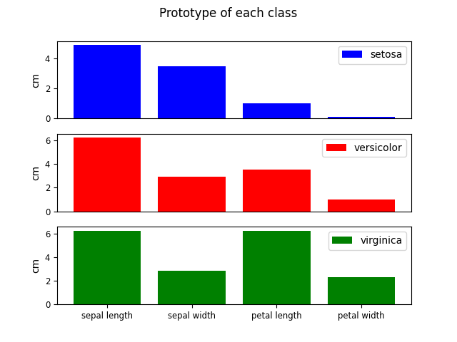
Extracting the Prototypes

The GLVQ model produces prototypes as representations for the different classes. These prototypes can be accessed and, e.g., plotted for visual inspection. Note that the prototypes of the model are within the z-score space and are transformed back before they are plotted.

colors = ["blue", "red", "green"]
num_prototypes = model.prototypes_.shape[0]
num_features = model.prototypes_.shape[1]

fig, ax = plt.subplots(num_prototypes, 1)
fig.suptitle("Prototype of each class")

for i, prototype in enumerate(model.prototypes_):
    # Reverse the z-transform to go back to the original feature space.
    prototype = scaler.inverse_transform(np.atleast_2d(prototype)).squeeze()

    ax[i].bar(
        range(num_features),
        prototype,
        color=colors[i],
        label=iris.target_names[model.prototypes_labels_[i]],
    )
    ax[i].set_xticks(range(num_features))
    if i == (num_prototypes - 1):
        ax[i].set_xticklabels([name[:-5] for name in iris.feature_names])
    else:
        ax[i].set_xticklabels([], visible=False)
        ax[i].tick_params(axis="x", which="both", bottom=False, top=False, labelbottom=False)
    ax[i].set_ylabel("cm")
    ax[i].legend()

References

[1] Sato, A., and Yamada, K. (1996) “Generalized Learning Vector Quantization.” Advances in Neural Network Information Processing Systems, 423–429, 1996.