Learning Behaviour

In these examples GMLVQ is used but the same applies to all the other algorithms. However, not each solver provides the same variables. Additionally, the options “lbfgs” and “bfgs” are implemented in scipy and their callbacks are different from the others. See Scipy’s documentation for further information.

import matplotlib
import matplotlib.pyplot as plt
import numpy as np
from sklearn.datasets import load_iris
from sklearn.metrics import classification_report
from sklearn.pipeline import make_pipeline
from sklearn.preprocessing import StandardScaler

from sklvq import GMLVQ

matplotlib.rc("xtick", labelsize="small")
matplotlib.rc("ytick", labelsize="small")

data, labels = load_iris(return_X_y=True)

We create a process logger object and provide it to the solver of the model.

class ProcessLogger:
    def __init__(self):
        self.states = np.array([])

    # A callback function has to accept two arguments, i.e., model and state, where model is the
    # current model, and state contains a number of the optimizers variables.
    def __call__(self, state):
        self.states = np.append(self.states, state)
        return False  # The callback function can also be used to stop training early,
        # if some condition is met by returning True.


# Initiate the "logger".
logger = ProcessLogger()

scaler = StandardScaler()

model = GMLVQ(
    distance_type="adaptive-squared-euclidean",
    activation_type="swish",
    activation_params={"beta": 2},
    solver_type="waypoint-gradient-descent",
    solver_params={
        "max_runs": 15,
        "k": 3,
        "step_size": np.array(
            [0.75, 0.85]
        ),  # Note we chose very large step_sizes here to show
        # the usefulness of waypoint averaging.
        "callback": logger,
    },
    random_state=1428,
)

pipeline = make_pipeline(scaler, model)

pipeline.fit(data, labels)

predicted_labels = pipeline.predict(data)

# Print a classification report (sklearn)
print(classification_report(labels, predicted_labels))

Out:

              precision    recall  f1-score   support

           0       1.00      1.00      1.00        50
           1       0.98      0.94      0.96        50
           2       0.94      0.98      0.96        50

    accuracy                           0.97       150
   macro avg       0.97      0.97      0.97       150
weighted avg       0.97      0.97      0.97       150

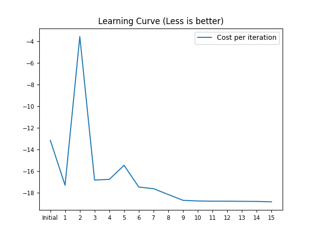
Additionally we can study the cost at each iteration of the solvers progress. Which doesn’t look very smooth and even gets worse. This is because of the chosen step_size, which is too large.

iteration, fun = zip(*[(state["nit"], state["fun"]) for state in logger.states])

ax = plt.axes()

ax.set_title("Learning Curve (Less is better)")
ax.plot(iteration, fun)
_ = ax.legend(["Cost per iteration"])

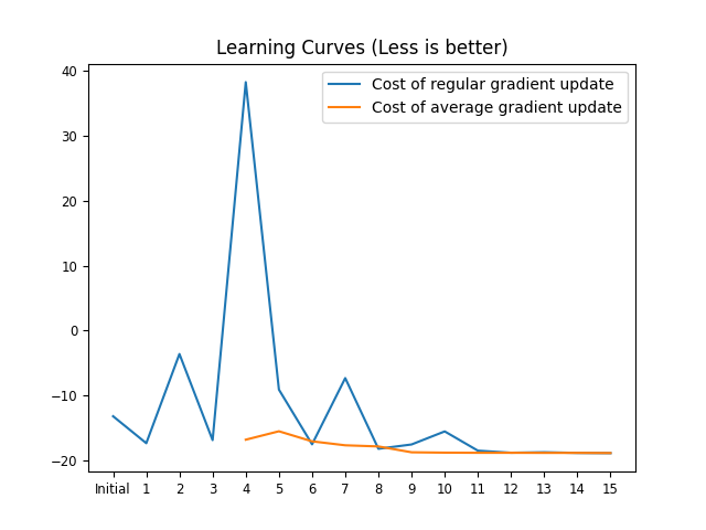
In the case of waypoint-gradient-descent there is an average cost (tfun) computed over the last k=3 updates and a regular update cost (nfun). Depending on which is less the regular update or the average update is applied.

tfun, nfun = zip(*[(state["tfun"], state["nfun"]) for state in logger.states])

ax = plt.axes()

ax.set_title("Learning Curves (Less is better)")
ax.plot(iteration, nfun)
ax.plot(iteration, tfun)
_ = ax.legend(["Cost of regular gradient update", "Cost of average gradient update"])