sklvq.solvers.AdaptiveMomentEstimation
-
class
sklvq.solvers.AdaptiveMomentEstimation(objective: sklvq.objectives._base.ObjectiveBaseClass, max_runs: int = 10, beta1: float = 0.9, beta2: float = 0.999, step_size: float = 0.001, epsilon: float = 0.0001, callback: Optional[callable] = None)[source]¶ Adaptive moment estimation (ADAM)
Implementation and description inspired by [1].
Adam maintains two moving averages of the gradient (
 ), which get updated for
every sample at each epoch/run until the maximum runs (
), which get updated for
every sample at each epoch/run until the maximum runs (max_runs) has been reached:![\mathbf{m} &= \beta_1 \cdot \mathbf{m} + (1 - \beta_1) \cdot \nabla e_i(\theta) \\
\mathbf{v} &= \beta_2 \cdot \mathbf{v} + (1 - \beta_2) \cdot [\nabla e_i(\theta)]^{\circ 2}.](../_images/math/a8e1f84c81ccfe71c72a902a39cdbad934b95481.png)
Since
 and
and  are initialized to zero vectors, they are biased towards zero.
To counteract this, unbiased estimates
are initialized to zero vectors, they are biased towards zero.
To counteract this, unbiased estimates  and
and  are computed:
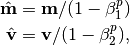
where
 is initially 0, but afterwards it’s increased by 1 each time before
selecting a new random sample. The unbiased estimates of the average gradient are then used
for the update step:
is initially 0, but afterwards it’s increased by 1 each time before
selecting a new random sample. The unbiased estimates of the average gradient are then used
for the update step: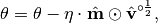
with
 the
the step_size. Additionally,beta1, andbeta2, can be chosen by the user.Note that
 denotes the elementwise (Hadamard) product and
  the elementwise power operation.
- Parameters
- objective: ObjectiveBaseClass, required
This is/should be set by the algorithm.
- max_runs: int
Number of runs over all the X. Should be >= 1
- beta1: float
Controls the decay rate of the moving average of the gradient. Should be < 1.0 and > 0.
- beta2: float
Controls the decay rate of the moving average of the squared gradient. Should be < 1.0 and > 0.
- step_size: float
The step size to control the learning rate.
- epsilon: float
Small value to overcome zero division
- callback: callable
Callable with signature callable(state). If the callable returns True the solver will stop (early). The state object contains the following information:
- “variables”
Concatenated 1D ndarray of the model’s parameters
- “nit”
The current iteration counter
- “fun”
The objective cost
- “m_hat”
Unbiased moving average of the gradient
- “v_hat”
Unbiased moving average of the Hadamard squared gradient
References
[1] LeKander, M., Biehl, M., & De Vries, H. (2017). “Empirical evaluation of gradient methods for matrix learning vector quantization.” 12th International Workshop on Self-Organizing Maps and Learning Vector Quantization, Clustering and Data Visualization, WSOM 2017.
-
solve(data: numpy.ndarray, labels: numpy.ndarray, model: LVQBaseClass)[source]¶ - Parameters
- datandarray of shape (number of observations, number of dimensions)
- labelsndarray of size (number of observations)
- modelLVQBaseClass
The initial model that will be changed and holds the results at the end